Saved Bookmarks
| 1. |
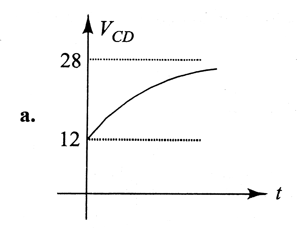
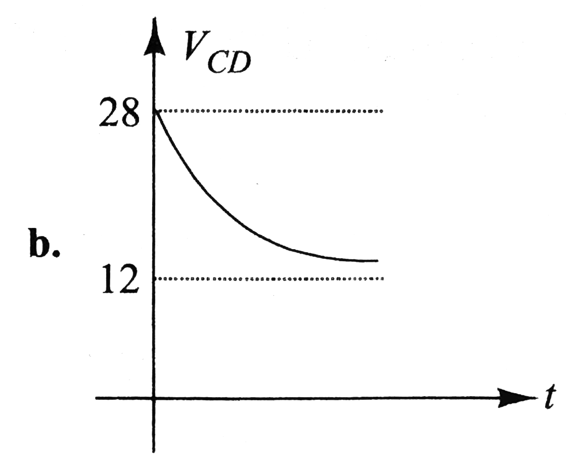
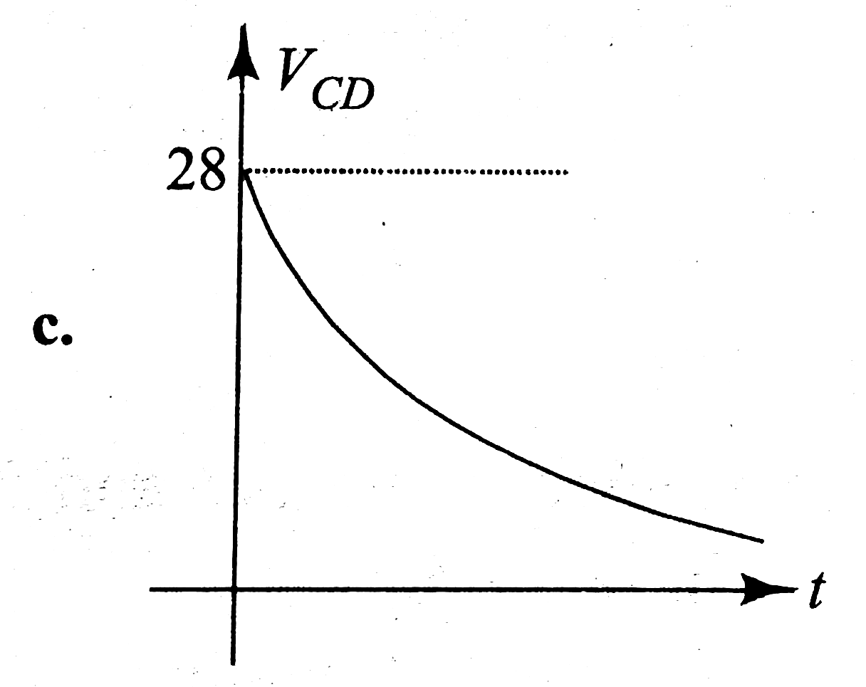
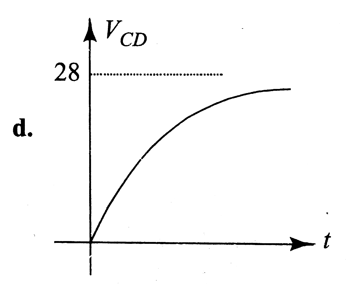
In Fig i_(1) = 10e^(-2t) A, i_(2) = 4 A, and V_(C) = 3e^(-2t) V. The variation of potential difference across C and D(V_(CD)) with time can be expressed as |
|
Answer»
`q = CV_(C) = (2)(3e^(-2t)) = 6e^(-2t) A` Current, `i_(C) = (dq)/(dt) = - 12e^(-2t)A` This current flows from `B` to `O`. From `KVL`, we have `i_(L) = i_(1) + i_(2) + i_(C) = 10e^(-2t) + 4 - 12e^(-2t)` `= (4 - 2t^(-2t)) A = [2 + 2(1 - E^(-2t))]A` `i_(L) vs`. time graph is as shows in Fig lt `i_(L)` increases from `2 A` to `4 A` expontially. 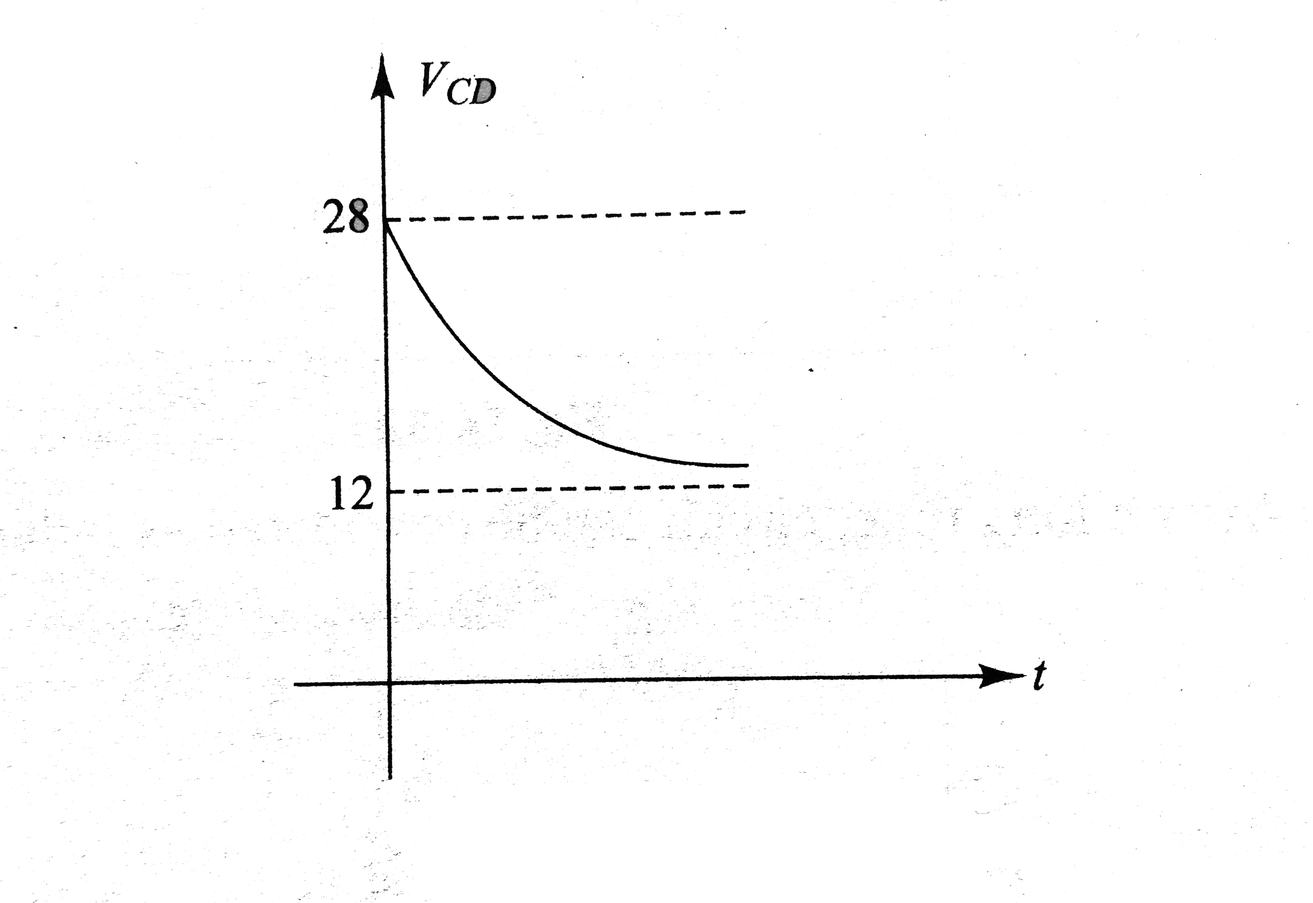 `V_(L) = L(di_(L))/(dt)` `= (4)(d)/(dt) (4 - 2e^(-2t)) = 16e^(-2t) V` `V_(L)` decreases exponentially from `16 A` to `0` as shows in Fig. To determine `V_(AC)`, we begin from `A` and at `C`. From `KVL`, we have 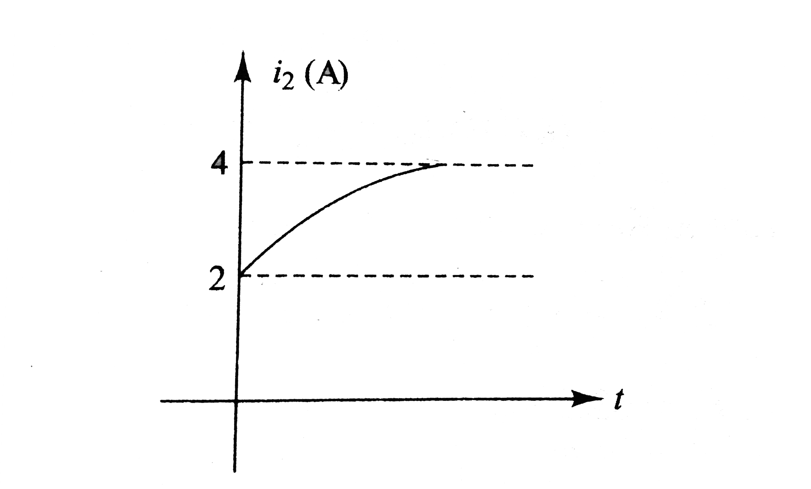 `V_(A) - i_(1)R_(1) + i_(2)R_(2) = V_(C)` `V_(A) - V_(C) = i_(1)R_(1) - i_(2)R_(2)` Substituting the values, we have `V_(AC) = (10 e^(-2t))(2) - (4)(3)` 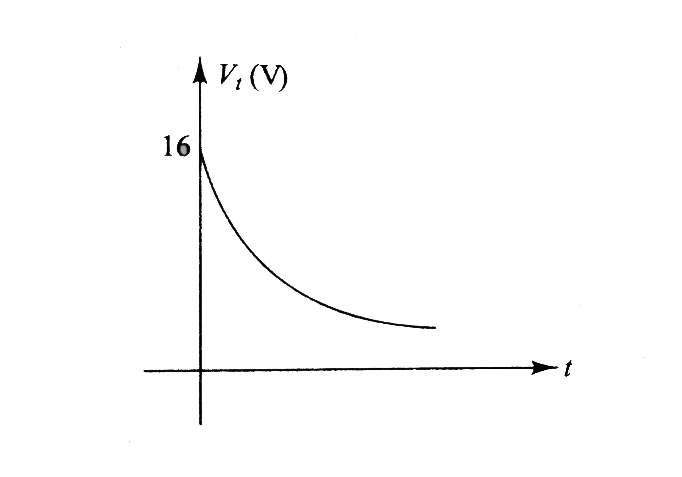 `V_(AC) = (20e^(-2t) - 12) V` At `t = 0`, `V_(AC) = 8V` At `t = oo`, `V_(AC) = - 12 V` Therefore, `V_(AC)` decrease exponentially from `8 V` to `12 V`. Similarly, we have from `A` to `B` `V_(A) - i_(1)R_(1) + V_(C) = V_(B)` `V_(AB) = V_(A) - V_(B) = i_(1)R_(1) - V_(C)` 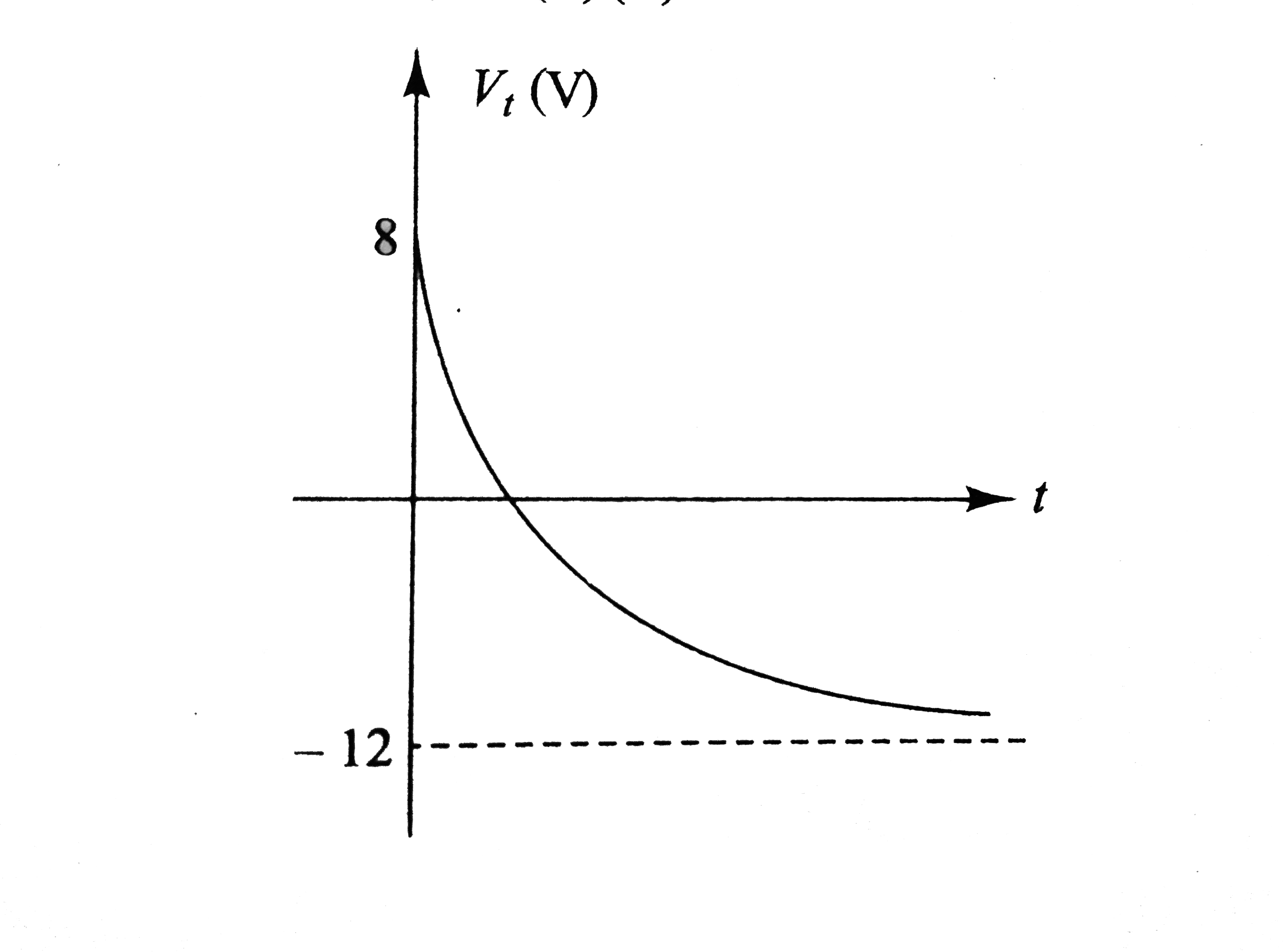 Substituting the values, we have `V_(AB)=^((10e^(-2t)))(2)-3e^(-2t)` `V_(AB) =^(17e^(-2t))V` Thus, `V_(AB)` decreases exponentially from `17 V` to `0`. As we move from `C` to `D`, `V_(C) - i_(2)R_(2) - V_(L) = V_(D)` `V_(CD)= V_(C) - V_(D) = i_(2)R_(2) + V_(L)` Substituting the values we have, `V_(CD)= (4)(3) + 16e^(-2t)` 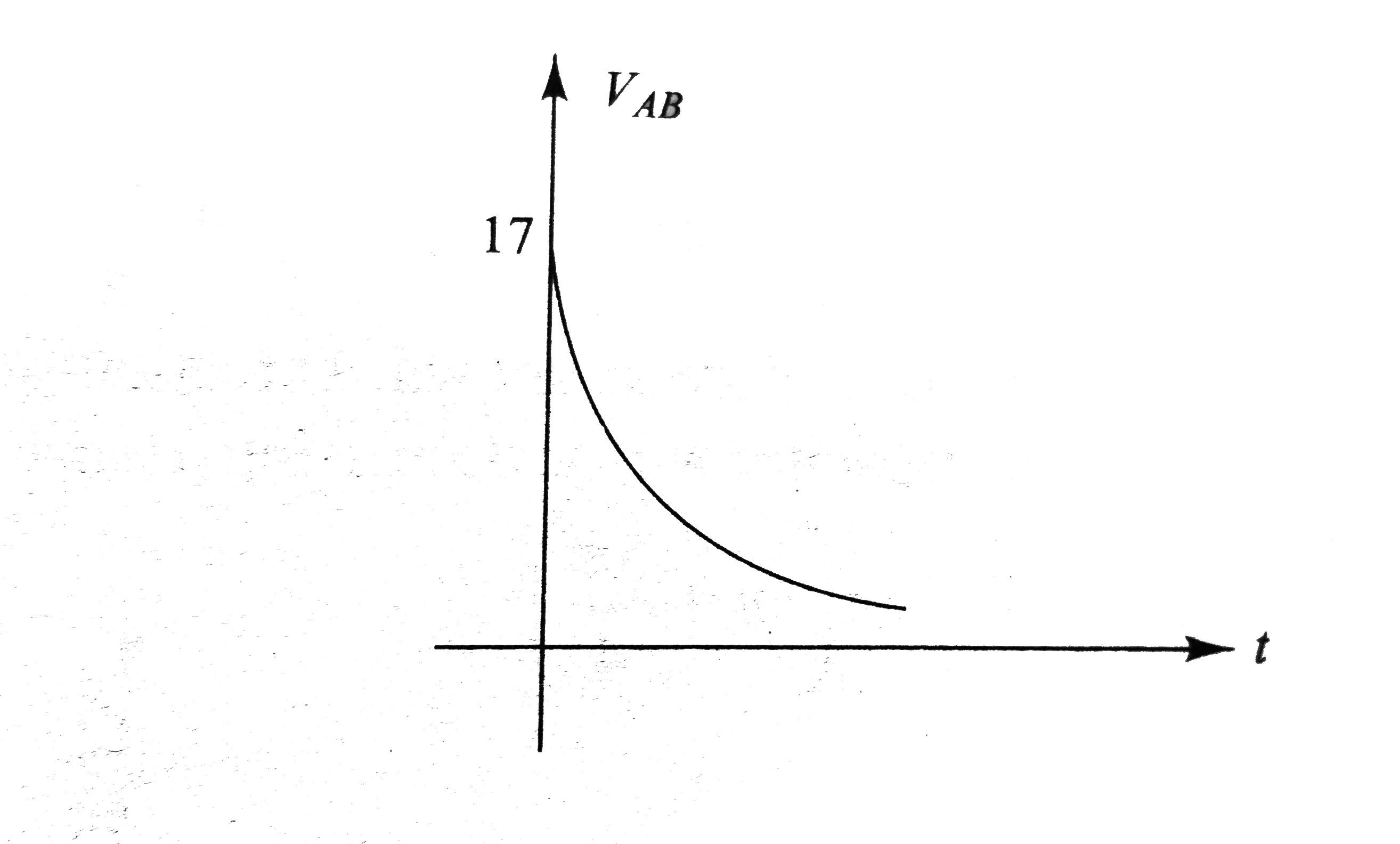 `V_(AD) = (12 + 16e^(-2t))V` At `t = 0, V_(CD) = 28 V` and at `t = oo, V_(CD) = 12 V` i.e., `V_(CD)` decreases exponentially from `28 V` to `12 V`. |
|